Linear Regression, Built by Hand on Advertising Data线性回归：用广告数据亲手推导

The setting is a consulting brief. A client sells one product in 200 markets and controls how much it spends on TV, radio and newspaper ads. Which spending actually moves sales, and by how much? The data is the advertising set from An Introduction to Statistical Learning.

One channel at a time. TV spending and sales correlate at 0.78. I derived the least-squares formulas for the slope and intercept, coded them directly, and got the same line from gradient descent and from scikit-learn. Each extra $1,000 of TV advertising goes with about 47 more units sold, and TV alone explains 61% of the variation in sales. The study then reads the output as a client would need it, from standard errors, t-values and p-values to a 95% confidence interval for the slope.

All three together. Fitted one at a time, every channel looks useful. Newspaper has a slope of about 0.056 and a p-value of 0.002. Fitted together, with least squares solved by matrix algebra, newspaper’s slope drops to about zero while TV and radio barely change, and the three-channel model explains 90% of the variation.

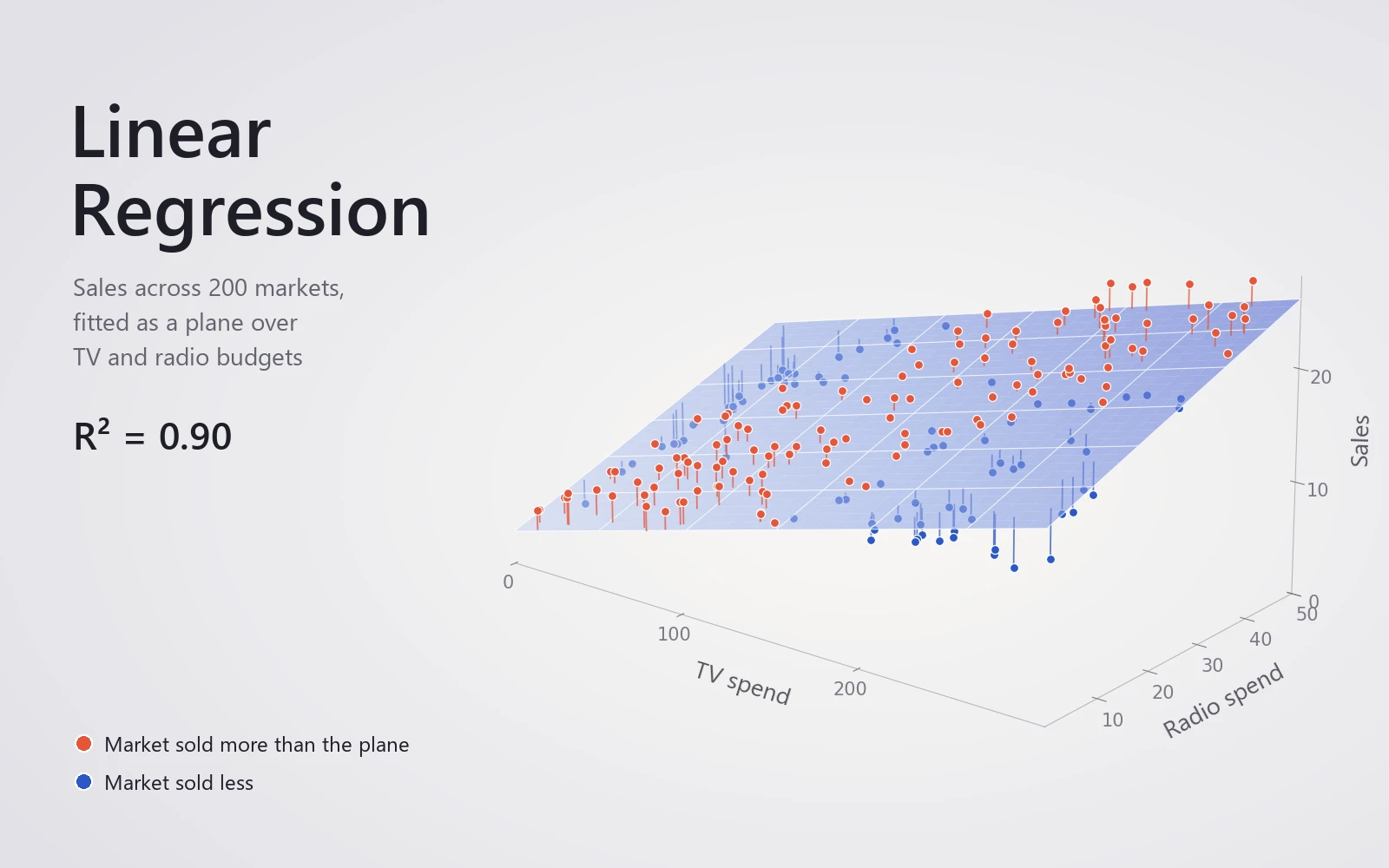
The reason is in the correlations. Markets that spend more on radio also tend to spend more on newspaper, at a correlation of 0.35, and radio does sell. On its own, newspaper takes credit for radio’s work. Dropping it costs nothing. The cover shows the model with TV and radio alone, a single plane through all 200 markets that still explains 90% of the variation.

The study goes on to an F-test for the whole model, forward and backward selection of channels, and the difference between a confidence interval for the average market and a prediction interval for a single one.

背景设定是一份咨询任务。一位客户在 200 个市场销售同一种产品，可以控制在电视、广播和报纸广告上各花多少钱。到底哪种投入真正带动了销量，又能带动多少？数据来自 An Introduction to Statistical Learning 中的广告数据集。

一次只看一个渠道。 电视广告投入和销量的相关系数为 0.78。我推导出斜率和截距的最小二乘公式，直接写成代码，再用梯度下降和 scikit-learn 分别拟合，得到的是同一条直线。电视广告每多投入 $1,000，销量大约多 47 件，单靠电视就能解释 61% 的销量变化。接着，研究按客户需要的方式解读输出结果，从标准误、t 值、p 值，一直到斜率的 95% 置信区间。

三个渠道一起看。 如果逐个单独拟合，每个渠道看起来都有用。报纸的斜率约为 0.056，p 值为 0.002。但把三个渠道放在一起拟合，用矩阵运算求解最小二乘，报纸的斜率就降到接近零，而电视和广播几乎不变，三渠道模型能解释 90% 的销量变化。

原因藏在相关性里。在广播上投入更多的市场，往往在报纸上也投入更多，两者的相关系数为 0.35，而广播确实能带来销量。单独看时，报纸把广播的功劳算到了自己头上。去掉报纸，模型毫无损失。封面图展示的是只用电视和广播的模型，一个平面穿过全部 200 个市场，依然能解释 90% 的销量变化。

研究还进一步讲了整个模型的 F 检验、渠道的前向和后向选择，以及针对平均市场的置信区间和针对单个市场的预测区间之间的区别。